Who is the best shooter in the NBA?

The full experience of sports

Any sports fan knows that sports data is a big part of the experience for the viewer. For ages, fans have been intertwined with the analytics of sport, i.e., the game performance of their favorite player, the goal difference of teams, and other interesting metrics. But data analysis in sports is now taking teams far beyond these old-school metrics and game performance. This is revealing the fact that some old-school metrics that have been reliable for ages may not show us the true meaning behind the numbers; like who is the best three-point shooter in the NBA?

Most people would imagine this as a simple math problem where we collect the records of all three-point shots taken by a player and divide the scoring total with the attempted total. This may seem like a good indicator of the best shooters but let’s look at how this logic falls through.

Where the old school method falls short

On one hand, we have Stephen Curry, arguably the best three-point shooter in the history of the NBA. Stephen Curry stands for his unwavering range from behind the arc with an impressive record of 185 three-points scored out of 434 three-point shots (42.4%). On the other hand, we have a young rookie talent, Aaron Gordon at Orlando Magic, who is totaling 9 successes out of 19 shots (47.4%).

Is Aaron Gordon (47.4%) better/more reliable at three-point shots than Stephen Curry (42.4%)? Saying something like that to an NBA fan would make you sound insane in the eyes of the fan. While Aaron Gordon has slightly higher percentages, there is not a lot of evidence: a typical player would score almost 34% of the time, and Gordon’s 47.4% success rate could be due to luck as we have a small sample size. Curry, on the other hand, has a lot of evidence to show that he is way above an average player.

How do we systematically compare and make a meaningful judgment about ratios like 185/434 vs. 9/19?

The simple solution could be to set some thresholds of shots taken and filter out the players who do not meet the minimum requirement. But that is far from ideal as we are throwing away valuable data. We want to somewhat measure the inherent three-point shot-taking ability of a player and since only looking at historical data doesn’t seem to do the trick; the task is to more accurately estimate his ability given his historical record.

Now let’s get data; NBA 2014-2015

I borrowed a dataset of all shots taken in the NBA league in the 2014-2015 season. The dataset is built around who shoots the shot and all explanatory variables adherent to that shot; like distance from the bucket, distance from the closest defender, time left on the shot clock, and so on.

Statistical models (made fun, I promise)

Prior (it’s like making a family betting odds for the NBA Finals game):

For this, we use something like Empirical Bayes. It’s kind of like using the results of the regular season games to predict the finals. Moreover, we will view the data after collection and estimate the prior distributions accordingly, yes, it’s a little bit of a cheeky cheat in the family bet game. However, this approach is used to take away some of the subjectivity that can alter the model since it is hard to get people to agree on a reasonable prior.

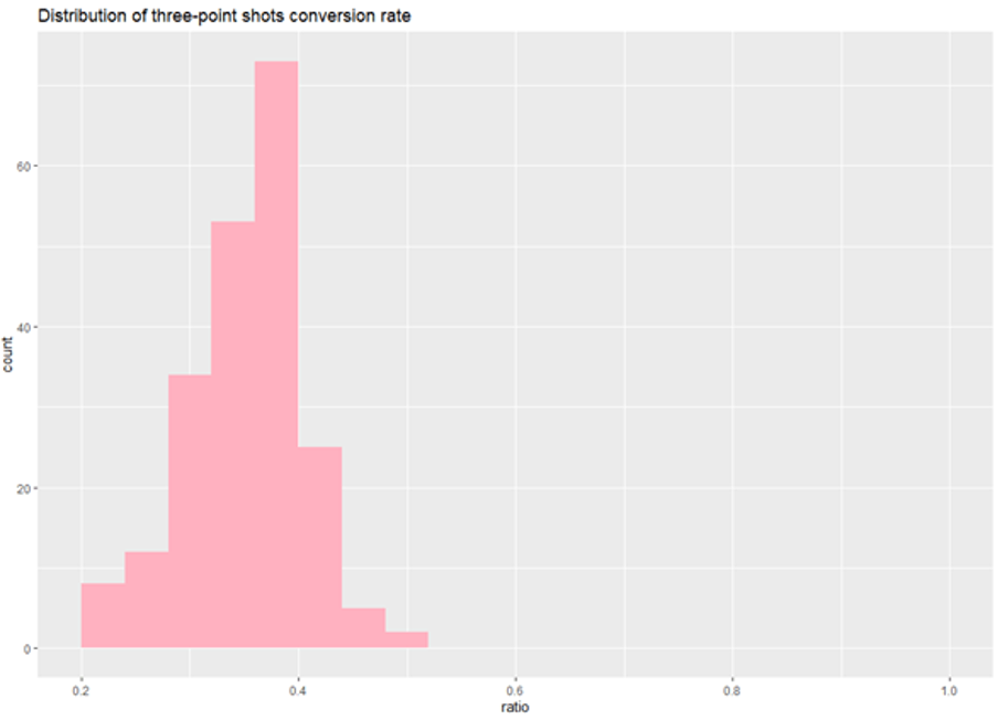
Figure 1: The actual distribution of shot conversion rate of three-point shots in the NBA

Distribution (It’s like putting ingredients in the oven)

The task of this section is to find a distribution that characterizes our empirical three-point shots ratio. Let me paint you a picture; you are in your element, listening to some awesome tunes in your underpants on a Sunday morning. Your feeling awesome after an awesome week and you just want to bake a cake. So, you start shoving some ingredients in a bowl, just from a feeling that it’s going to become a wonderful cake. But you’re not a baker, so you don’t really know what the ingredients are going to become in the oven. So, you lower the music and look at the ingredients and you make an educated guess that it’s going to become a carrot cake. So, you add some fleeced carrot to the bowl and put it in the oven.

That’s what we did with the data. So, we have a feeling that it’s going to represent the data pretty well. The beta distribution is handy in the sense that it has a domain from 0 to 1 and it’s flexible, in the sense that it could represent what we see in our histogram. WAIT, WAIT, WAIT… Back to Sunday morning, so if it makes a pretty awesome carrot cake, we blast the music again and make the white cream and eat the cake whole. And in the same sense, if we see that the Beta distribution makes our Bayesian calculation easier when we combine with the likelihood from the binomial distribution, we (the nerd gang) sit back in our Razor game chair, reach for the victory bag of Doritos and crack open a frosty mountain dew.

Which ultimately, we did. The result is a posterior distribution which is also a Beta distribution of a precise form Beta(alpha + H, beta + M). Or in cake terms means that we are going to have a carrot cake with slight additions of chocolate chips (marked in alpha and beta. WHICH IS AWESOME.

Empirical prior:

For the sake of the article, I’m going to skip the calculations of The Beta distribution to our conversion rate but if you trust me, the estimation is alpha = 16.8 and beta = 31.9.

Let see how well this estimation fits our data:

Figure 2: Beta distribution of shot conversion rate of three-point shots in the NBA: α = 16.8 and β = 31.9

Creating a distribution for every player in the NBA

So, we have made the cake… and so we slice it up and make a lot of muffins. The muffins represent the (posterior) distributions for each player’s conversion rate using the method described here above. That is a Beta distribution of the form Beta(alpha + H, beta + M), where H and M are the numbers of hits and misses, respectively. Here the alpha and beta are the chocolate chips that we added to make the cake a little bit more awesome.

The posterior mean for a specific player (i) will be:

For example, the posterior distribution mean for Curry and Gordon‘s three-point shot conversion rate will be:

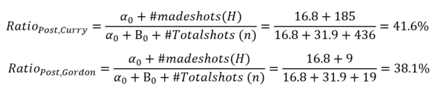
We can plot their posteriors distributions (with some other players) as follows:

It can be seen that Curry‘s strong records result in a very high posterior mean and a narrow credible interval, while Aaron Gordon‘s posterior mean conversion has a larger credible interval, as he has fewer data to stand for. Meanwhile, Derrick Rose is just not that good when it comes to taking three-point shots and the same goes for Brook Lopez as with Aaron Gordon, posterior mean conversion has a larger credible interval, as he has fewer data to stand for.

The top 10 3pt shooters:

After applying the empirical Bayes estimate and beta-binomial posterior calculation, the results for the top 10 three-point shooters in the NBA 2014-2015, are as follows:

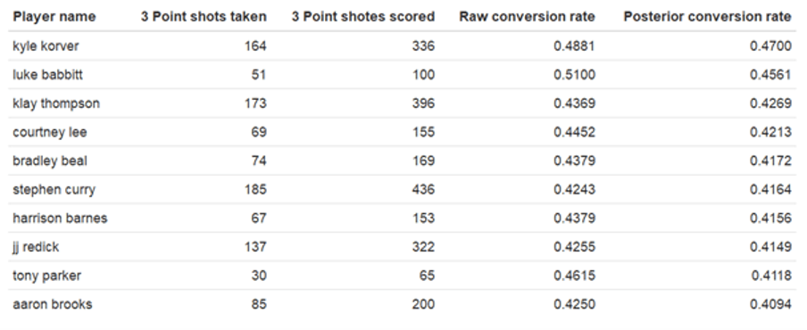
It turns out that the best three-point shooters, at least by this method, are Kyle Korver, Luke Babbitt, and Klay Thompson. Interestingly, we can see that for these players, their conversion rates shrink after we apply this procedure. We can plot the original and the adjusted ratios on a plot to assess the adjustment.

Conclusion:

Using the concept of empirical Bayesian estimation: we can leverage the overall distribution of our data before arriving at a more realistic estimate of each average. Then, we used the concept of conjugate priors to bypass the complications of calculating the posterior distributions in our procedure. 

For this article, I have conveniently ignored many complications.